size, bs =128, 32dls = get_dls(size, bs)print(f'{len(dls.train_ds)} training images, {len(dls.valid_ds)} validation images, 'f'{len(dls.vocab)} classes, at {size} pixels')
9469 training images, 3925 validation images, 10 classes, at 128 pixels
print(f'torch {torch.__version__} | {torch.get_num_threads()} CPU threads | 'f'training on {default_device()}')
torch 2.9.1+cu128 | 24 CPU threads | training on cuda:0
Let’s start with a bit of context for the purpose of the demonstration. Imagine that we want to deploy a VGG16 model on a mobile device that has limited storage capacity and that our task requires our model to run sufficiently fast. It is known that parameters and speed efficiency are not the strong points of VGG16 but let’s see what we can do with it.
Let’s first check the number of parameters and the inference time of VGG16.
Model Size: 537.30 MB (disk), 134318423 parameters
So our model has 134 millions parameters and needs 537.30MB of disk space in order to be stored.
x, y = dls.one_batch()
baseline_ms, lo, hi = evaluate_cpu_speed(learn.model, x[0][None])print(f'Inference Speed: {baseline_ms:.2f}ms ({lo:.2f}–{hi:.2f} over three repeats)')
Inference Speed: 23.40ms (23.34–23.52 over three repeats)
And it takes 23.40ms to perform inference on a single image.
Note
Measured on an Intel i9-14900KS, at the thread count and torch version printed above, one image at a time, ten warm-up passes then three timing repeats of fifty passes each, reported as the mean with the min and max of the three. Every latency on this page comes from that same single run, at the 1-minute load averages the recap prints.
Snap ! This is more than we can afford for deployment, ideally we would like our model to take only half of that…but should we give up ? Nope, there are actually a lot of techniques that we can use to help reducing the size and improve the speed of our models! Let’s see how to apply them with FasterAI.
We will first train our VGG16 model to have a baseline of what performance we should expect from it.
set_seed(42, reproducible=True)with learn.no_bar(), learn.no_logging(): learn.fit_one_cycle(10, 1e-4)baseline_k, baseline_n = report_accuracy(learn.model, 'VGG16', dls)trained_ms, lo, hi = evaluate_cpu_speed(learn.model, x[0][None])print(f'Inference Speed: {trained_ms:.2f}ms ({lo:.2f}–{hi:.2f} over three repeats)')
VGG16 accuracy: 3183/3925 (81.10%)
Inference Speed: 23.84ms (23.82–23.87 over three repeats)
Ten epochs from scratch leave it at 81.10% (3183/3925 correct on the validation set), and the trained model takes 23.84ms on that same single image. Those are the two numbers every step below is read against.
So we would like our network to have comparable accuracy but fewer parameters and running faster… And the first technique that we will show how to use is called Knowledge Distillation
Knowledge Distillation
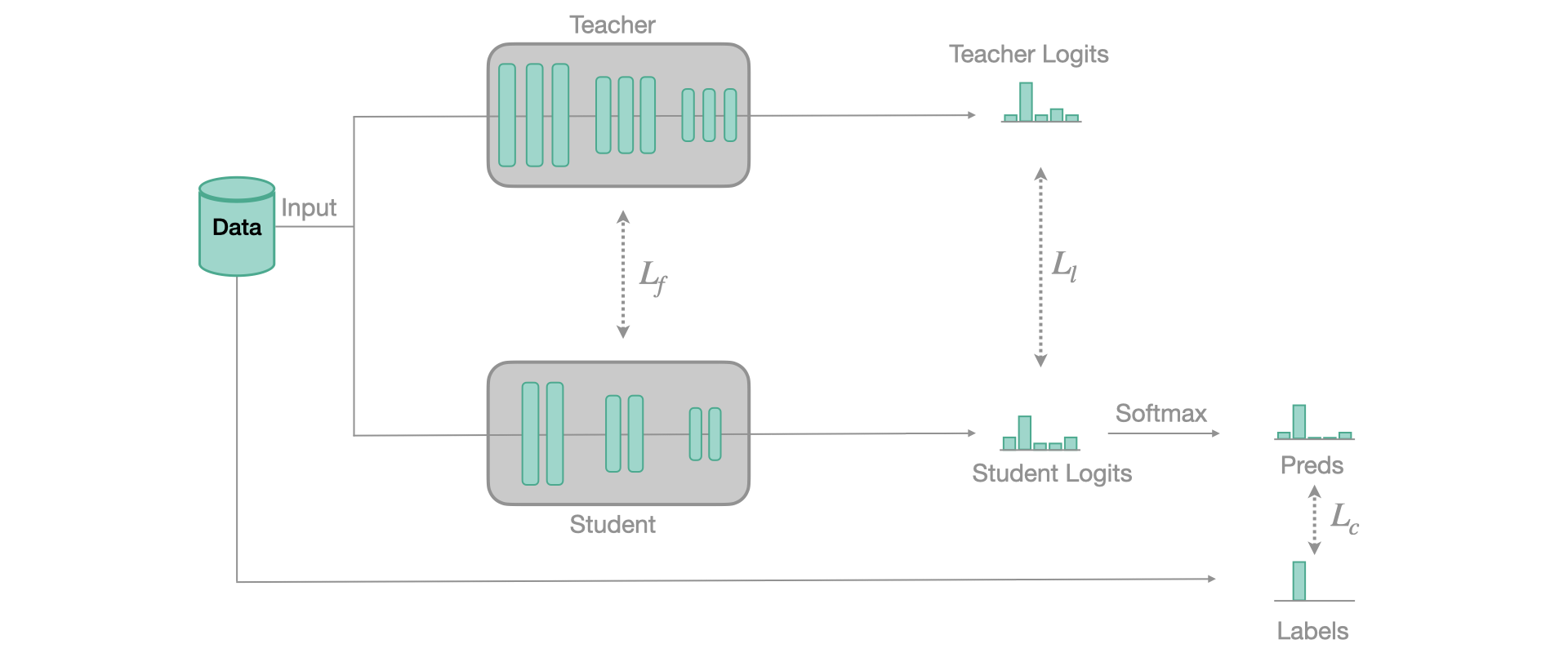
Knowledge distillation is a simple yet very efficient way to train a model. It was introduced in 2006 by Caruana et al.. The main idea behind is to use a small model (called the student) to approximate the function learned by a larger and high-performing model (called the teacher). This can be done by using the large model to pseudo-label the data. This idea has been used very recently to break the state-of-the-art accuracy on ImageNet.
When we train our model for classification, we usually use a softmax as last layer. This softmax has the particularity to squish low value logits towards 0, and the highest logit towards 1. This has the effect of completely losing all the inter-class information, or what is sometimes called the dark knowledge. This is the information that is valuable and that we want to transfer from the teacher to the student.
To do so, we still use a regular classification loss but at the same time, we’ll use another loss, computed between the softened logits of the teacher (our soft labels) and the softened logits of the student (our soft predictions). Those soft values are obtained when you use a soft-softmax, that avoids squishing the values at its output. Our implementation follows this paper and the basic principle of training is represented in the figure below:
To use Knowledge Distillation with FasterAI, you only need to use this callback when training your student model:
KnowledgeDistillationCallback(teacher, loss)
You only need to give to the callback the model of your teacher and the distillation loss to use. Behind the scenes, FasterAI will take care of making your model train using knowledge distillation.
from fasterai.distill.allimport*
The first thing to do is to find a teacher, which can be any model, that preferrably performs well. We will chose VGG19 for our demonstration. To make sure it performs better than our VGG16 model, let’s start from a pretrained version.
Our teacher has 93.55% of accuracy (3672/3925) which is pretty good, it is ready to take a student under its wing. So let’s create our student model and train it with the Knowledge Distillation callback:
VGG16 student accuracy: 3200/3925 (81.53%)
Difference with the vanilla VGG16: 17 images
With the teacher, the student ends at 81.53% (3200/3925) against 81.10% (3183/3925) for the vanilla VGG16 — same ten epochs, same learning rate, same seed, one run each. That is 17 images. One run of each does not say whether that gap survives another seed, so this page does not attribute it to the distillation.
With some experimentations we could come up with a model smaller than VGG16 but able to reach the same performance as our baseline! You can try to find it by yourself later, but for now let’s continue with the next technique !
Sparsifying
Now that we have a student model in hand, we have some room to compress it. And we’ll start by making the network sparse. As explained in a previous article, there are many ways leading to a sparse network.
Note
Usually, the process of making a network sparse is called Pruning. I prefer using the term Pruning when parameters are actually removed from the network, which we will do in the next section.
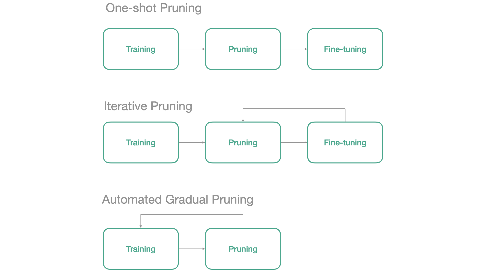
In FasterAI, the sparsification is managed by a callback, that will replace the least important parameters of your model by zeroes during the training, following the schedule you hand it — the Automated Gradual Pruning of the figure above is one of those, and it removes parameters as the model trains, so it doesn’t require to pretrain the model. The callback has a wide variety of parameters to tune your Sparsifying operation, let’s take a look at them:
sparsity: the amount of sparsity that you want in your network, as a fraction in [0, 1] (0.5 = 50%)
granularity: on what granularity you want the sparsification to be operated
context: either local or global, will affect the selection of parameters to be choosen in each layer independently (local) or on the whole network (global).
criteria: the criteria used to select which parameters to remove, from fasterai.core.criteria (large_final, movement, random, …)
schedule: which schedule you want to follow for the sparsification, from fasterai.core.schedule (one_shot, iterative, agp, one_cycle, cos, lin)
But let’s come back to our example!
Here, we will make our network 50% sparse, and remove entire filters, selected globally and based on their final magnitude. We will train with a learning rate a bit smaller to be gentle with our network because it has already been trained. The scheduling selected is cosinusoidal, so the sparsification starts and ends quite slowly.
Sparsifying filter until a sparsity of 50.00%
Saving Weights at epoch 0
Sparsity at the end of epoch 0: 1.22%
Sparsity at the end of epoch 1: 4.77%
Sparsity at the end of epoch 2: 10.31%
Sparsity at the end of epoch 3: 17.27%
Sparsity at the end of epoch 4: 25.00%
Sparsity at the end of epoch 5: 32.73%
Sparsity at the end of epoch 6: 39.69%
Sparsity at the end of epoch 7: 45.23%
Sparsity at the end of epoch 8: 48.78%
Sparsity at the end of epoch 9: 50.00%
Final Sparsity: 50.00%

Sparsity Report:
--------------------------------------------------------------------------------
Layer                          Type            Params     Zeros      Sparsity
--------------------------------------------------------------------------------
features.0                     Conv2d          1,728      0              0.00%
features.3                     Conv2d          36,864     0              0.00%
features.7                     Conv2d          73,728     0              0.00%
features.10                    Conv2d          147,456    0              0.00%
features.14                    Conv2d          294,912    0              0.00%
features.17                    Conv2d          589,824    0              0.00%
features.20                    Conv2d          589,824    0              0.00%
features.24                    Conv2d          1,179,648  783,360       66.41%
features.27                    Conv2d          2,359,296  1,723,392     73.05%
features.30                    Conv2d          2,359,296  1,681,920     71.29%
features.34                    Conv2d          2,359,296  1,626,624     68.95%
features.37                    Conv2d          2,359,296  1,608,192     68.16%
features.40                    Conv2d          2,359,296  1,520,640     64.45%
--------------------------------------------------------------------------------
Overall                        all             14,710,464 8,944,128     60.80%
VGG16 sparsified accuracy: 3154/3925 (80.36%)
Our network now has 50% of its filters composed entirely of zeroes, and it ends at 80.36% (3154/3925) against 81.53% (3200/3925) before the sparsification — one run each. Read the report above rather than that single figure: the sparsity is spread very unevenly, because a global context compares the filters of the whole network against each other, and here the first seven convolutions kept all of theirs. Obviously, choosing a higher sparsity makes it more difficult for the network to keep a similar accuracy. Other parameters can also widely change the behaviour of our sparsification process. For example choosing a more fine-grained sparsity picks the weights one by one instead of by whole filters, which is then more difficult to take advantage of in terms of speed.
Let’s now see how much we gained in terms of speed. Because we removed 50% of convolution filters, we should expect crazy speed-up right ?
sparse_ms, lo, hi = evaluate_cpu_speed(student.model, x[0][None])print(f'Inference Speed: {sparse_ms:.2f}ms ({lo:.2f}–{hi:.2f} over three repeats)')
Inference Speed: 24.56ms (24.54–24.58 over three repeats)
Well actually, no: 24.56ms, against 23.40ms for the dense model, single run each. We didn’t remove any parameters, we just replaced some by zeroes, remember? The amount of parameters is still the same:
Model Size: 537.30 MB (disk), 134318423 parameters
Which leads us to the next section.
Pruning
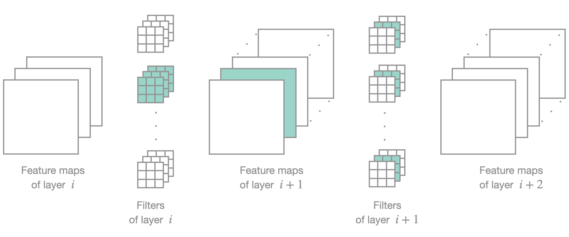
Why don’t we see any acceleration even though we zeroed half of the filters? That’s because natively, our hardware does not know that our matrices are sparse and thus isn’t able to accelerate the computation. The easiest work around, is to physically remove filters — most of the ones we zeroed, since the pruner selects its own half. But this operation requires to change the architecture of the network.
This pruning only works if we remove entire filters as it is the only case where we can change the architecture accordingly. Hopefully, sparse computations are making their way into common deep learning librairies so this section may become useless in the future.
pruning_ratio: the amount of filters to remove, as a fraction in [0, 1] (0.5 = 50%)
schedule: which schedule you want to follow for the pruning, from fasterai.core.schedule
context: either local or global, will affect the selection of filters to be choosen in each layer independently (local) or on the whole network (global).
criteria: the criteria used to select which filters to remove, from fasterai.core.criteria
Ignoring output layer: classifier.6
Total ignored layers: 1
Pruning ratio at the end of epoch 0: 1.94%
Pruning ratio at the end of epoch 1: 19.96%
Pruning ratio at the end of epoch 2: 45.82%
Pruning ratio at the end of epoch 3: 49.74%
Pruning ratio at the end of epoch 4: 50.00%
VGG16 pruned accuracy: 3158/3925 (80.46%)
pruned_ms, lo, hi = evaluate_cpu_speed(student.model, x[0][None])print(f'Inference Speed: {pruned_ms:.2f}ms ({lo:.2f}–{hi:.2f} over three repeats)')
Inference Speed: 14.60ms (14.58–14.62 over three repeats)
Yay ! Now we can talk ! The filters are gone for real this time — 43481770 parameters left against 134318423 with the same filters merely zeroed, and 14.60ms against 24.56ms, single run each. And the accuracy printed above says we didn’t mess up somewhere: 80.46% (3158/3925) at the end of the pruning fit.
And there is actually more that we can do ! Let’s keep going !
Batch Normalization Folding
Batch Normalization Folding is a really easy to implement and straightforward idea. The gist is that batch normalization is nothing more than a normalization of the input data at each layer. Moreover, at inference time, the batch statistics used for this normalization are fixed. We can thus incorporate the normalization process directly in the convolution by changing its weights and completely remove the batch normalization layers, which is a gain both in terms of parameters and in terms of computations. For a more in-depth explaination, see this blog post.
This is how to use it with FasterAI:
bn_folder = BN_Folder()
bn_folder.fold(model)
Again, you only need to pass your model and FasterAI takes care of the rest. For models built using the nn.Sequential, you don’t need to change anything. For others, if you want to see speedup and compression, you actually need to subclass your model to remove the batch norm from the parameters and from the forward method of your network.
Note
This operation is lossless in exact arithmetic, as it redefines the convolution to take batch norm into account and is thus equivalent. In float32 it left the count of correct predictions where it was, 3158/3925 before and after.
The parameters drop is generally not that significant, especially in a network such as VGG where almost all parameters are contained in the FC layers but, hey, any gain is good to take.
Now that we removed the batch normalization layers, we should again see a speedup.
folded_ms, lo, hi = evaluate_cpu_speed(folded_model, x[0][None])print(f'Inference Speed: {folded_ms:.2f}ms ({lo:.2f}–{hi:.2f} over three repeats)')
Inference Speed: 12.29ms (12.29–12.30 over three repeats)
12.29ms, against 14.60ms before the fold, single run each.
Again, let’s double check that we didn’t mess up somewhere:
folded_learner = Learner(dls, folded_model, metrics=[accuracy])folded_k, folded_n = report_accuracy(folded_learner.model, 'VGG16 folded', dls)print(f'Correct predictions moved by the fold: {folded_k - pruned_k}')
VGG16 folded accuracy: 3158/3925 (80.46%)
Correct predictions moved by the fold: 0
And we’re still not done yet ! As we know for VGG16, most of the parameters are comprised in the fully-connected layers so there should be something that we can do about it, right ?
FC Layers Factorization
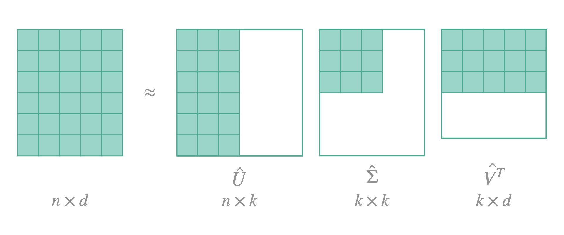
We can indeed, factorize our big fully-connected layers and replace them by an approximation of two smaller layers. The idea is to make an SVD decomposition of the weight matrix, which will express the original matrix in a product of 3 matrices: \(U \Sigma V^T\). With \(\Sigma\) being a diagonal matrix with non-negative values along its diagonal (the singular values). We then define a value \(k\) of singular values to keep and modify matrices \(U\) and \(V^T\) accordingly. The resulting will be an approximation of the initial matrix.
In FasterAI, to decompose the fully-connected layers of your model, here is what you need to do:
decomposed_ms, lo, hi = evaluate_cpu_speed(decomposed_model, x[0][None])print(f'Inference Speed: {decomposed_ms:.2f}ms ({lo:.2f}–{hi:.2f} over three repeats)')
Inference Speed: 10.93ms (10.91–10.96 over three repeats)
The parameters go from 43470249 down to 26243247, and the timing from 12.29ms to 10.93ms, single run each. This is thus a matter of compromise between network weight and speed, and here both went the same way.
However, this technique is an approximation so it is not lossless, so we should retrain our network a bit to recover its performance.
This operation reaches whatever a network keeps in its fully-connected layers, and more recent architectures usually do not keep that many parameters there.
Quantization
from fasterai.quantize.allimport*
Now that we have removed every superfluous parameter that we could, we can still continue to compress our model. A common way to do so is now to reduce the precision of each parameter in the network, making it considerably smaller. Such an approach is called Quantization and won’t affect the total number of parameter but will make each one of them smaller to store, and have the network compute in 8-bit integers instead of floats.
In FasterAI, quantization can be done in a static way, i.e. apply quantization to the model, also called Post-Training Quantization. It also can be applied during training, also called Quantization-Aware Training. The callback below does the second one: it swaps the layers for their observed counterparts before the fit, trains through them, and converts the result to an actual 8-bit model afterwards.
QuantizeCallback(backend='x86')
The backend is the engine the quantized model will run on; x86 is the CPU one, and the model that comes out of the fit runs on the CPU, which is where we measure it.
The model that comes out of the fit is an 8-bit one, and it scores 79.62% (3125/3925) after five more epochs, against 77.96% (3060/3925) for the floating-point model those epochs started from — one run each, two things changed at once.
quantized_ms, lo, hi = evaluate_cpu_speed(final_learner.model, x[0][None])print(f'Inference Speed: {quantized_ms:.2f}ms ({lo:.2f}–{hi:.2f} over three repeats)')
Inference Speed: 7.99ms (7.33–9.29 over three repeats)
The count barely moves — 26243287 against 26243247, the few extra ones being the scales the quantized layers carry — but each parameter is now stored on 8 bits instead of 32, so the model takes 26.42 MB against 104.98 MB. And it runs in 7.99ms against 10.93ms for the floating-point model it was converted from, single run each.
Extra Acceleration
One last thing, which compresses nothing but takes what we have and hands it to the CPU in the shape it likes: a channels-last memory layout and a traced graph, so the Python overhead of the module tree is gone at inference time.
from fasterai.misc.cpu_optimizer import optimize_for_cpu
26.52 MB, against 26.42 MB for the state dict of the same model. And in terms of speed:
accelerated_ms, lo, hi = evaluate_cpu_speed(final_model, x[0][None])print(f'Inference Speed: {accelerated_ms:.2f}ms ({lo:.2f}–{hi:.2f} over three repeats)')
Inference Speed: 6.38ms (6.36–6.41 over three repeats)
6.38ms, against 7.99ms for the same weights run eagerly in the default memory layout, single run each.
Again, let’s double check that we didn’t mess up somewhere:
traced_k, traced_n = report_accuracy(final_model, 'VGG16 traced', dls)trace_agree = count_agreement(final_learner.model, final_model, dls)print(f'predictions identical on {trace_agree} of {traced_n} images')
VGG16 traced accuracy: 3125/3925 (79.62%)
predictions identical on 3925 of 3925 images
3125/3925, the same count as the model it was traced from, and the two answer identically on all 3925 validation images: the tracing changed the memory layout and the call path, not the arithmetic.
Summary
So to recap, we saw in this article how to use fasterai to: 1. Make a student model learn from a teacher model (Knowledge Distillation) 2. Make our network sparse (Sparsifying) 3. Optionally physically remove the zero-filters (Pruning) 4. Remove the batch norm layers (Batch Normalization Folding) 5. Approximate our big fully-connected layers by smaller ones (Fully-Connected Layers Factorization) 6. Quantize the model to reduce the precision of the weights (Quantization) 7. Trace the result to take the Python overhead out of the inference (Extra Acceleration)
print(f"VGG16 after its ten epochs: {baseline_size/1e6:.2f} MB and {trained_ms:.2f}ms per image "f"({baseline_k}/{baseline_n} correct)")print(f"After the seven steps: {accelerated_size/1e6:.2f} MB and {accelerated_ms:.2f}ms per image "f"({traced_k}/{traced_n} correct)")print(f"Compression ratio: {baseline_size/accelerated_size:.1f}x, "f"speed ratio: {trained_ms/accelerated_ms:.1f}x")print(f"1-minute load average at the timing cells: from {min(LOADS):.1f} to {max(LOADS):.1f}")
VGG16 after its ten epochs: 537.30 MB and 23.84ms per image (3183/3925 correct)
After the seven steps: 26.52 MB and 6.38ms per image (3125/3925 correct)
Compression ratio: 20.3x, speed ratio: 3.7x
1-minute load average at the timing cells: from 0.5 to 9.2
And we saw that by applying those, we could reduce our VGG16 model from 537.30 MB of parameters down to 26.52 MB (20.3x compression) — that last figure written by torch.jit.save, where every other size on this page is a torch.save of the state dict — and also speed-up the inference from 23.84ms to 6.38ms (3.7x speed-up), single run, the reference being the trained VGG16 and not the untrained one timed at the top. The accuracy went from 3183/3925 correct to 3125/3925 — the final model having had thirty-five epochs to the baseline’s ten (see the scope below).
Scope. VGG16 trained from scratch on Imagenette at 128 pixels, 9469 training images and 3925 validation ones, one run of each step: ten epochs for the baseline, three for the pretrained VGG19 teacher, ten for the student, ten with the SparsifyCallback, five with the PruneCallback, five to recover from the factorization and five more with the QuantizeCallback. The baseline and the student are built and fitted under set_seed(42, reproducible=True), so those two differ only in the callback; nothing else on the page is seeded. Every accuracy on this page is the whole validation set, printed as k/n. Every latency is a single image on the CPU of the box named above, ten warm-up passes then three timing repeats of fifty passes each, one run of the page; the recap prints the range of the 1-minute load average at those cells, 0.5 to 9.2.
Note
Please keep in mind that the techniques presented above are not magic 🧙♂️, so do not expect to see the same compression and speed-up everytime. What you can achieve highly depend on the architecture that you are using (some are already speed/parameter efficient by design) or the task it is doing (some datasets are so easy that you can remove almost all your network without seeing a drop in performance)
See Also
Knowledge Distillation - The distillation callback, its losses and its feature-map variants
Sparsify Callback - Sparsification on its own, granularity by granularity
Prune Callback - Removing the filters inside the training loop
BatchNorm Folding - Folding BatchNorm into the convolution ahead of it