Schedules

Make your neural network sparse with fastai

Neural Network Pruning usually follows one of the next 3 schedules:

In fasterai, all those 3 schedules can be applied from the same callback. We’ll cover each below

In the SparsifyCallback, there are several parameters to ‘shape’ our pruning schedule: * start_sparsity: the initial sparsity of our model, generally kept at 0 as after initialization, our weights are generally non-zero. * end_sparsity: the target sparsity at the end of the training * start_epoch: we can decide to start pruning right from the beginning or let it train a bit before removing weights. * sched_func: this is where the general shape of the schedule is specified as it specifies how the sparsity evolves along the training. You can either use a schedule available in fastai our even coming with your own !

path = untar_data(URLs.PETS)

files = get_image_files(path/"images")

def label_func(f): return f[0].isupper()

device = 'cuda:0' if torch.cuda.is_available() else 'cpu'

dls = ImageDataLoaders.from_name_func(path, files, label_func, item_tfms=Resize(64), device=device)

We will first train a network without any pruning, which will serve as a baseline.

learn = vision_learner(dls, resnet18, metrics=accuracy)
learn.unfreeze()

learn.fit_one_cycle(10)

epoch	train_loss	valid_loss	accuracy	time
0	0.773334	0.612048	0.803112	00:03
1	0.484909	0.651635	0.823410	00:04
2	0.275744	0.470824	0.819350	00:04
3	0.210518	0.255528	0.896482	00:04
4	0.187754	0.402981	0.848444	00:04
5	0.168017	0.282024	0.878214	00:04
6	0.104045	0.215567	0.923545	00:04
7	0.063283	0.211051	0.928281	00:04
8	0.032446	0.187703	0.937754	00:04
9	0.021794	0.190525	0.938430	00:04

One-Shot Pruning

The simplest way to perform pruning is called One-Shot Pruning. It consists of the following three steps:

You first need to train a network
You then need to remove some weights (depending on your criteria, needs,…)
You fine-tune the remaining weights to recover from the loss of parameters.

With fasterai, this is really easy to do. Let’s illustrate it by an example:

learn = vision_learner(dls, resnet18, metrics=accuracy)
learn.unfreeze()

In this case, your network needs to be trained before pruning. This training can be done independently from the pruning callback, or simulated by the start_epoch that will delay the pruning process.

You thus only need to create the Callback with the one_shot schedule and set the start_epoch argument, i.e. how many epochs you want to train your network before pruning it.

sp_cb=SparsifyCallback(sparsity=90, granularity='weight', context='local', criteria=large_final, schedule=one_shot)

Let’s start pruningn after 3 epochs and train our model for 6 epochs to have the same total amount of training as before

learn.fit(10, cbs=sp_cb)

Pruning of weight until a sparsity of 90%
Saving Weights at epoch 0

epoch	train_loss	valid_loss	accuracy	time
0	0.579104	0.326434	0.863329	00:04
1	0.365433	0.696673	0.757104	00:04
2	0.272263	0.507063	0.830853	00:04
3	0.222548	0.264393	0.892422	00:05
4	0.180488	0.251536	0.896482	00:04
5	0.225195	0.280325	0.879567	00:04
6	0.163019	0.266747	0.906631	00:04
7	0.122460	0.255492	0.905277	00:04
8	0.100369	0.287000	0.895805	00:04
9	0.073793	0.272262	0.908660	00:04

Sparsity at the end of epoch 0: 0.00%
Sparsity at the end of epoch 1: 0.00%
Sparsity at the end of epoch 2: 0.00%
Sparsity at the end of epoch 3: 0.00%
Sparsity at the end of epoch 4: 90.00%
Sparsity at the end of epoch 5: 90.00%
Sparsity at the end of epoch 6: 90.00%
Sparsity at the end of epoch 7: 90.00%
Sparsity at the end of epoch 8: 90.00%
Sparsity at the end of epoch 9: 90.00%
Final Sparsity: 90.00%

Sparsity Report:
--------------------------------------------------------------------------------
Layer                          Type            Params     Zeros      Sparsity  
--------------------------------------------------------------------------------
0.0                            Conv2d          9,408      8,467         90.00%
0.4.0.conv1                    Conv2d          36,864     33,177        90.00%
0.4.0.conv2                    Conv2d          36,864     33,177        90.00%
0.4.1.conv1                    Conv2d          36,864     33,177        90.00%
0.4.1.conv2                    Conv2d          36,864     33,177        90.00%
0.5.0.conv1                    Conv2d          73,728     66,355        90.00%
0.5.0.conv2                    Conv2d          147,456    132,710       90.00%
0.5.0.downsample.0             Conv2d          8,192      7,372         89.99%
0.5.1.conv1                    Conv2d          147,456    132,710       90.00%
0.5.1.conv2                    Conv2d          147,456    132,710       90.00%
0.6.0.conv1                    Conv2d          294,912    265,420       90.00%
0.6.0.conv2                    Conv2d          589,824    530,841       90.00%
0.6.0.downsample.0             Conv2d          32,768     29,491        90.00%
0.6.1.conv1                    Conv2d          589,824    530,841       90.00%
0.6.1.conv2                    Conv2d          589,824    530,841       90.00%
0.7.0.conv1                    Conv2d          1,179,648  1,061,683     90.00%
0.7.0.conv2                    Conv2d          2,359,296  2,123,366     90.00%
0.7.0.downsample.0             Conv2d          131,072    117,964       90.00%
0.7.1.conv1                    Conv2d          2,359,296  2,123,366     90.00%
0.7.1.conv2                    Conv2d          2,359,296  2,123,366     90.00%
--------------------------------------------------------------------------------
Overall                        all             11,166,912 10,050,211    90.00%

Iterative Pruning

Researchers have come up with a better way to do pruning than pruning all the weigths in once (as in One-Shot Pruning). The idea is to perform several iterations of pruning and fine-tuning and is thus called Iterative Pruning.

You first need to train a network
You then need to remove a part of the weights weights (depending on your criteria, needs,…)
You fine-tune the remaining weights to recover from the loss of parameters.
Back to step 2.

learn = vision_learner(dls, resnet18, metrics=accuracy)
learn.unfreeze()

In this case, your network needs to be trained before pruning.

You only need to create the Callback with the iterative schedule and set the start_epoch argument, i.e. how many epochs you want to train your network before pruning it.

The iterative schedules has a n_stepsparameter, i.e. how many iterations of pruning/fine-tuning you want to perform. To modify its value, we can use the partial function like this:

iterative = partial(iterative, n_steps=5)

sp_cb=SparsifyCallback(sparsity=90, granularity='weight', context='local', criteria=large_final, schedule=iterative)

Let’s start pruningn after 3 epochs and train our model for 6 epochs to have the same total amount of training as before

learn.fit(10, cbs=sp_cb)

Pruning of weight until a sparsity of 90%
Saving Weights at epoch 0

epoch	train_loss	valid_loss	accuracy	time
0	0.540534	0.429058	0.818674	00:04
1	0.343884	0.275153	0.872124	00:04
2	0.246214	0.325832	0.870771	00:03
3	0.188388	0.760273	0.748985	00:03
4	0.161098	0.326967	0.879567	00:03
5	0.120742	0.337820	0.878890	00:03
6	0.108090	0.260159	0.901894	00:03
7	0.255249	0.327174	0.863329	00:03
8	0.163483	0.272866	0.888363	00:03
9	0.112936	0.243970	0.911367	00:03

Sparsity at the end of epoch 0: 0.00%
Sparsity at the end of epoch 1: 0.00%
Sparsity at the end of epoch 2: 30.00%
Sparsity at the end of epoch 3: 30.00%
Sparsity at the end of epoch 4: 60.00%
Sparsity at the end of epoch 5: 60.00%
Sparsity at the end of epoch 6: 60.00%
Sparsity at the end of epoch 7: 90.00%
Sparsity at the end of epoch 8: 90.00%
Sparsity at the end of epoch 9: 90.00%
Final Sparsity: 90.00%

Sparsity Report:
--------------------------------------------------------------------------------
Layer                          Type            Params     Zeros      Sparsity  
--------------------------------------------------------------------------------
0.0                            Conv2d          9,408      8,467         90.00%
0.4.0.conv1                    Conv2d          36,864     33,177        90.00%
0.4.0.conv2                    Conv2d          36,864     33,177        90.00%
0.4.1.conv1                    Conv2d          36,864     33,177        90.00%
0.4.1.conv2                    Conv2d          36,864     33,177        90.00%
0.5.0.conv1                    Conv2d          73,728     66,355        90.00%
0.5.0.conv2                    Conv2d          147,456    132,710       90.00%
0.5.0.downsample.0             Conv2d          8,192      7,372         89.99%
0.5.1.conv1                    Conv2d          147,456    132,710       90.00%
0.5.1.conv2                    Conv2d          147,456    132,710       90.00%
0.6.0.conv1                    Conv2d          294,912    265,420       90.00%
0.6.0.conv2                    Conv2d          589,824    530,841       90.00%
0.6.0.downsample.0             Conv2d          32,768     29,491        90.00%
0.6.1.conv1                    Conv2d          589,824    530,841       90.00%
0.6.1.conv2                    Conv2d          589,824    530,841       90.00%
0.7.0.conv1                    Conv2d          1,179,648  1,061,682     90.00%
0.7.0.conv2                    Conv2d          2,359,296  2,123,365     90.00%
0.7.0.downsample.0             Conv2d          131,072    117,964       90.00%
0.7.1.conv1                    Conv2d          2,359,296  2,123,366     90.00%
0.7.1.conv2                    Conv2d          2,359,296  2,123,366     90.00%
--------------------------------------------------------------------------------
Overall                        all             11,166,912 10,050,209    90.00%

Gradual Pruning

Here is for example how to implement the Automated Gradual Pruning schedule.

learn = vision_learner(dls, resnet18, metrics=accuracy)
learn.unfreeze()

sp_cb=SparsifyCallback(sparsity=90, granularity='weight', context='local', criteria=large_final, schedule=agp)

Let’s start pruning after 3 epochs and train our model for 6 epochs to have the same total amount of training as before

learn.fit(10, cbs=sp_cb)

Pruning of weight until a sparsity of 90%
Saving Weights at epoch 0

epoch	train_loss	valid_loss	accuracy	time
0	0.614568	0.392339	0.836265	00:05
1	0.381756	0.379407	0.847091	00:04
2	0.273133	0.325403	0.844384	00:04
3	0.225977	0.302057	0.874154	00:04
4	0.186390	0.251494	0.891746	00:04
5	0.155119	0.322763	0.865359	00:04
6	0.158356	0.303624	0.878890	00:04
7	0.131190	0.241102	0.902571	00:06
8	0.121991	0.238827	0.912043	00:06
9	0.081199	0.237045	0.918133	00:06

Sparsity at the end of epoch 0: 0.00%
Sparsity at the end of epoch 1: 0.00%
Sparsity at the end of epoch 2: 29.71%
Sparsity at the end of epoch 3: 52.03%
Sparsity at the end of epoch 4: 68.03%
Sparsity at the end of epoch 5: 78.75%
Sparsity at the end of epoch 6: 85.25%
Sparsity at the end of epoch 7: 88.59%
Sparsity at the end of epoch 8: 89.82%
Sparsity at the end of epoch 9: 90.00%
Final Sparsity: 90.00%

Sparsity Report:
--------------------------------------------------------------------------------
Layer                          Type            Params     Zeros      Sparsity  
--------------------------------------------------------------------------------
0.0                            Conv2d          9,408      8,467         90.00%
0.4.0.conv1                    Conv2d          36,864     33,177        90.00%
0.4.0.conv2                    Conv2d          36,864     33,177        90.00%
0.4.1.conv1                    Conv2d          36,864     33,177        90.00%
0.4.1.conv2                    Conv2d          36,864     33,177        90.00%
0.5.0.conv1                    Conv2d          73,728     66,355        90.00%
0.5.0.conv2                    Conv2d          147,456    132,710       90.00%
0.5.0.downsample.0             Conv2d          8,192      7,372         89.99%
0.5.1.conv1                    Conv2d          147,456    132,710       90.00%
0.5.1.conv2                    Conv2d          147,456    132,710       90.00%
0.6.0.conv1                    Conv2d          294,912    265,420       90.00%
0.6.0.conv2                    Conv2d          589,824    530,841       90.00%
0.6.0.downsample.0             Conv2d          32,768     29,491        90.00%
0.6.1.conv1                    Conv2d          589,824    530,841       90.00%
0.6.1.conv2                    Conv2d          589,824    530,841       90.00%
0.7.0.conv1                    Conv2d          1,179,648  1,061,683     90.00%
0.7.0.conv2                    Conv2d          2,359,296  2,123,366     90.00%
0.7.0.downsample.0             Conv2d          131,072    117,964       90.00%
0.7.1.conv1                    Conv2d          2,359,296  2,123,366     90.00%
0.7.1.conv2                    Conv2d          2,359,296  2,123,366     90.00%
--------------------------------------------------------------------------------
Overall                        all             11,166,912 10,050,211    90.00%

Even though they are often considered as different pruning methods, those 3 schedules can be captured by the same Callback. Here is how the sparsity in the network evolves for those methods;

Let’s take an example here. Let’s say that we want to train our network for 3 epochs without pruning and then 7 epochs with pruning.

Then this is what our different pruning schedules will look like:

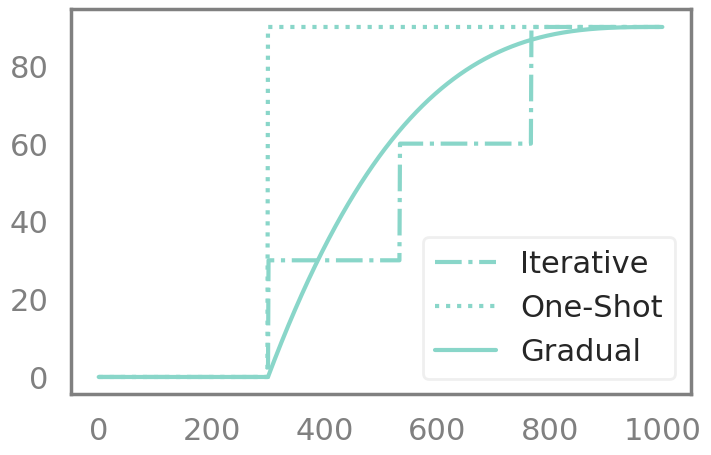
You can also come up with your own pruning schedule !

Summary

Schedule	Behavior
`one_shot`	Apply once at a set point
`iterative`	Step-wise pruning in N discrete steps
`agp`	Automated Gradual Pruning (cubic decay)
`one_cycle`	Logistic-function based single cycle
`cos`	Cosine annealing
`lin`	Linear ramp
`dsd`	Dense-Sparse-Dense (prune then regrow)

One-Shot Pruning

Iterative Pruning

Gradual Pruning

Summary

See Also